现有的分类方法一般都需要训练样本集,训练样本的类别是实现知道的,理想情况下,一个 classifier 会从它得到的训练集中进行“学习”,从而具备对未知数据进行分类的能力,这种提供训练数据的过程通常叫做 supervised learning (监督学习)。但在实际应用中,训练样本集的标签很有可能无法得到。聚类算法,按照大量未知类别数据中内在的特性进行分类,把特性彼此接近的归入同一类,而把特性不相似的点分到不同的类中去。这在 Machine Learning 中被称作 unsupervised learning (无监督学习)。
距离及相似性度量参见距离度量。显然对于同一数据集选用不同的相似性度量,得到的结果也是不同的。
一、 聚类准则
离差平方和准则:设共有N个样本向量(欧式意义下),分成K个群 ,每个群有
,每个群有 个样本,其中心
 。则所有属于第
 个群的样本点和该群中心点距离平方和为
 ,
,  个群的类内离差平方和为

依照这个准则,一般应把 分到离它最近的中心所代表的类中去,否则
 将会变大。这在各类自然地聚成团,团内较紧密,团间距离较大的场合很合适。这个函数,其中
  在数据点
在数据点  被归类到 cluster k 的时候为 1 ,否则为 0 。

我们的目标是寻找 和 来最小化,但是这里有两个未知量。因此我们采用Alternate Minimization的思想,即固定一个,优化另一个。下一步则固定优化得到的量,再优化另一个参数。
令固定,将对求导并令导数等于0,易得当最小的时候应满足

也就是说 的值应当是被分配到 cluster k 中的所有数据点的平均值(这也是K-means的由来)。由于每一次迭代都是取到 的最小值,因此 只会不断地减小(或者不变),而不会增加,这保证了 k-means 最终会到达一个极小值。虽然 k-means 并不能保证总是能得到全局最优解。
二、动态聚类算法
1、K-means
K-means算法的基本思想就是极小化离差平方和,在具体实现方法上,采用逐次迭代修正的办法。先选定中心个数K并作初始分类,然后不断改变样本在K类中的划分及K个中心的位置,达到使离差平方和J为极小。
k-means聚类算法的流程如下:
初始化 1. 随机初始化聚类中心 。可以考虑把最初K个样本指定为K个中心。
赋值步骤 2. a. 对与每一个聚类中心,计算所有样本到该聚类中心的距离,然后选出距离该聚类中心最近的几个样本作为一类;

即某个样本  属于哪一类,取决于该样本距离哪一个聚类中心最近。
出现平局怎么办?我们不希望一个数据点到两个均值有相同的距离。但是如果发生了,总是设为较小的类k。
更新步骤 b. 对上面分成的k类,根据类里面的样本,重新估计该类的中心:(batch version)

c. 重复a和b直至收敛对于新的聚类中心。若 对于所有
对于所有 成立,即迭代修正以后没有改变任何点的分类情况及中心位置,则称算法收敛。
|
1 2 3 4 5 6 7 8 |
while !converged for each point assign label end for each cluster compute mean end end |
k-means收敛性证明:
根据k-means的算法,可以看出,(a) 是固定聚类中心,选择该类的样本,(b) 是样本固定,调整聚类中心,即每次都是固定一个变量,调整另一个变量。(这就是字典学习K-svd等算法的alternate minimization思想。)k-means完全是在针对离差平方和 坐标上升,这样, 必然是单调递减,所以的值必然收敛。在理论上,这种方法可能会使得k-means在一些聚类结果之间产生震荡,即几组不同的
 和
和  有着相同的失真函数值,但是这种情况在实际情况中很少出现。
由于准则函数是一个非凸函数,所以坐标上升不能保证该函数全局收敛,即准则函数容易陷入局部收敛。但是大多数情况下,k-means都可以产生不错的结果,如果担心陷入局部收敛,可以多运行几次k-means(采用不同的随机初始聚类中心),然后从多次结果中选出失真函数最小的聚类结果。
值得注意的是,K-means算法常被用来初始化GMM模型的参数,在使用EM算法前。
关于k-means算法的缺陷讨论:
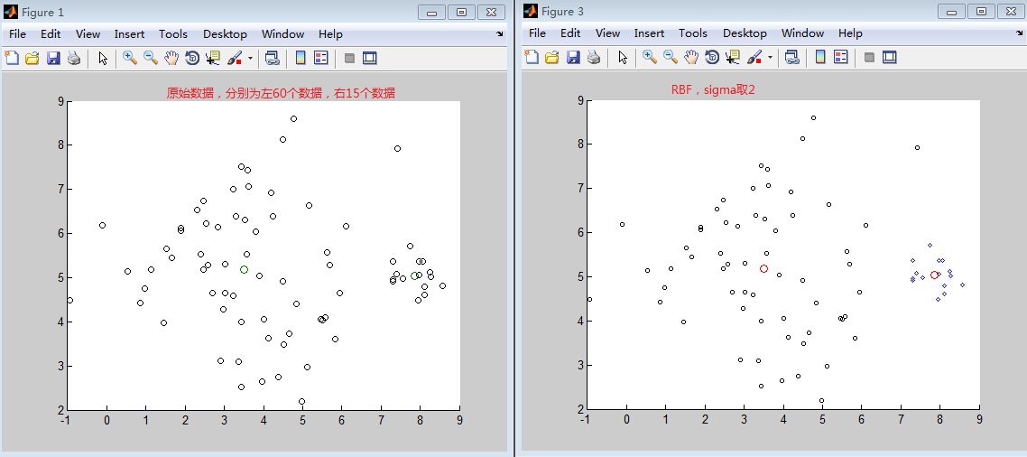
1)如图由两个高斯分布混合所产生的75个数据点集合。右边的高斯具有较小权重(只有1/5的数据点),是较窄的类。利用具有K=2个均值的K-均值聚类的结果。4个属于大类的数据点被分配到小类,而两个均值都移到了聚类真实中心的左边。(不平衡类)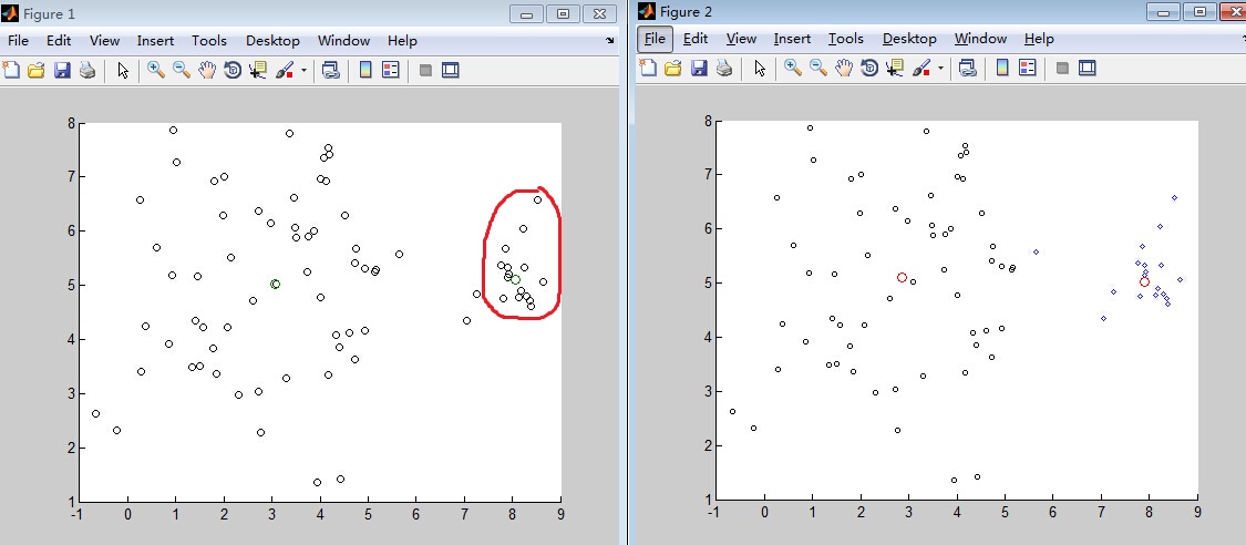
|
1 2 3 4 5 6 7 8 9 10 11 12 13 14 15 16 17 18 19 20 21 22 23 24 25 26 27 28 29 30 31 32 |
% An example of unbalanced class cluster % Author: Hui Ni % Mail: kiminh@sjtu.edu.cn clc,clear all; N = 75 ; x = [ ones(N*4/5,1) * [3,5] ] ; x = 1.75*randn(size(x)) + x ; xx = [ ones(N/5,1) * [8,5] ] ; xx = 0.35*randn(size(xx)) + xx ; X = [ x ; xx ] ; m=[mean(x);mean(xx)]; scatter(X(:,1),X(:,2),30,'ko'); hold on scatter(m(:,1),m(:,2)); [Idx,C]=kmeans(X,2); idx1=find(Idx==1); idx2=find(Idx==2); cluster1=X(idx1,:); cluster2=X(idx2,:); figure; scatter(cluster1(:,1),cluster1(:,2),10,'d'); hold on scatter(cluster2(:,1),cluster2(:,2),10,'ko'); m_bar=[mean(cluster1);mean(cluster2)]; hold on scatter(m_bar(:,1),m(:,2)); |
K-均值算法只考虑数据点之间的距离;每个类的权重或宽度都没有得到表示。因此,实际上属于宽类的数据点被错误地划分到了窄类。
有没有办法可以解决这个问题呢?试了一下核函数的方法,分别为线性核和RBF核。不过也是碰巧感觉,没有真正解决。后面试了几次又都失败了。当然比K-means效果是要好很多的。到底怎么解决有待研究。
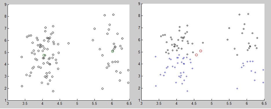
2)K-means也没有办法表示类的形状。数据点显然属于两个延长类,但是K-means却把它分成了两半。这说明了一个问题:K-means均值中的距离d是存在一些问题的。
|
1 2 3 4 5 6 7 8 9 10 11 12 13 14 15 16 17 18 19 20 21 22 23 24 25 26 27 28 29 30 31 32 33 34 |
%Author: Hu Ni %Mail:kiminh@sjtu.edu.cn clc,clear all; off = 1.0 ; M = [0.25 0;0 1.5] ; N = 100 ; x = [ ones(N*0.7,1) * [5-off,5] ] ; x = randn(size(x))*M + x ; xx = [ ones(N*0.3,1) * [5+off,5] ] ; xx = randn(size(xx))*M + xx ; X= [ x ; xx ] ; m=[mean(x);mean(xx)]; scatter(X(:,1),X(:,2),30,'ko'); hold on scatter(m(:,1),m(:,2)); [Idx,C]=kmeans(X,2); idx1=find(Idx==1); idx2=find(Idx==2); cluster1=X(idx1,:); cluster2=X(idx2,:); figure; scatter(cluster1(:,1),cluster1(:,2),10,'d'); hold on scatter(cluster2(:,1),cluster2(:,2),10,'ko'); m_bar=[mean(cluster1);mean(cluster2)]; hold on scatter(m_bar(:,1),m(:,2)); |
3)K-means算法是一个“硬”的而不是“软”的算法,这是说点只会被分配到一个类中,分配到一个类的搜有点对于这个类而言都是等价的。但是,我们知道在决定点似应被分配到所有类的位置时,位于两个或多个类的边界上的点只起到部分作用。在K-means算法中,每个边界上的点都分配到一个类中,在其他类中没有发言权。
算法复杂度分析:其时间复杂度为O(NKT),N为训练样本数,K是类别个数,T为迭代次数。
上述batch version是对所有类中心进行更新,算法复杂度比较高。
随机逼近算法和序列学习(Sequential Estimation)
序列学习方法允许数据点在一个时刻被处理一次然后被丢弃,这对于在线学习的实时性非常重要。(PRML 2.3.5)
对于高斯分布的最大似然估计,均值参数可以被估计为

在观察 个数据点后,通过
 估计。然后,观察
 个数据点,对于估计
 作一些小的修正,令其旧的估计移动一小部分,沿着“误差信号”方向
 ,比例为
,比例为 。显然这同batch version得到的结果是一致的。
Robbins-Monro
更为一般的推导,详见PRML2.3.5
K-means的Stochastic 版本
对于训练样本集中的每个数据点 ,计算该样本与聚类中心的欧式距离,并更新最近的聚类中心

其中,代表距离数据点最近的聚类标号。 为学习率,MacQueen将其设为
 ,其中
,其中 为分配到该聚类的样本数。
待研究。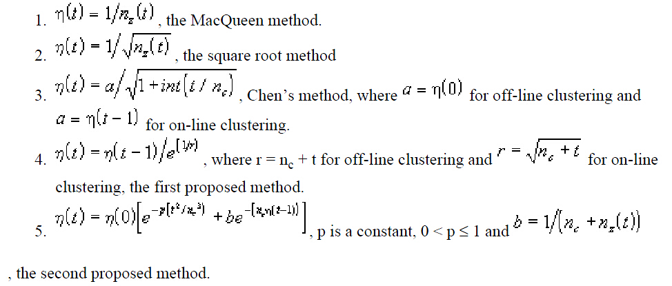
相关习题:
1)假设数据点 来自单一可分的二维高斯分布,其均值为0,方差为
 。探讨软K-均值算法的特性。设K=2,假设N很大,当
 发生变化时,研究算法的不动点。
2、K-medoids
k-medoids 可以算是 k-means 的一个变种。k-medoids 和 k-means 不一样的地方在于中心点的选取。
然而在 k-medoids 中,我们将中心点的选取限制在当前 cluster 所包含的数据点的集合中。换句话说,在 k-medoids 算法中,我们将从当前 cluster 中选取这样一个点——它到其他所有(当前 cluster 中的)点的距离之和最小——作为中心点。k-means 和 k-medoids 之间的差异就类似于一个数据样本的均值 (mean) 和中位数 (median) 之间的差异:前者的取值范围可以是连续空间中的任意值,而后者只能在给样本给定的那些点里面选。
这么做的好处:在 k-medoids 中,我们把原来的目标函数 中的欧氏距离改为一个任意的 dissimilarity measure 函数  :
:
最常见的方式是构造一个 dissimilarity matrix  来代表 ,其中的元素
  表示第
表示第  只狗和第
只狗和第  只狗之间的差异程度,例如,两只 Samoyed 之间的差异可以设为 0 ,一只 German Shepherd Dog 和一只 Rough Collie 之间的差异是 0.7,和一只 Miniature Schnauzer 之间的差异是 1 ,等等。
除此之外,由于中心点是在已有的数据点里面选取的,因此相对于 k-means 来说,不容易受到那些由于误差之类的原因产生的 Outlier 的影响,更加 robust 一些。
从 k-means 变到 k-medoids ,时间复杂度陡然增加了许多:在 k-means 中只要求一个平均值  即可,而在 k-medoids 中则需要枚举每个点,并求出它到所有其他点的距离之和,复杂度为
  。
。
|
1 2 3 4 5 6 7 8 9 10 11 12 13 14 15 16 17 18 |
function [label, energy, index] = kmedoids(X,k) % X: d x n data matrix % k: number of cluster % Written by Mo Chen (sth4nth@gmail.com) v = dot(X,X,1);//1*2000,计算X训练样本中每个样本的内积 D = bsxfun(@plus,v,v')-2*(X'*X);//2000*2000,这是一个对称阵,对角线元素为0 n = size(X,2); [~, label] = min(D(randsample(n,k),:),[],1); last = 0; while any(label ~= last) [~, index] = min(D*sparse(1:n,label,1,n,k,n),[],1);//选取3个类中心 last = label; [val, label] = min(D(index,:),[],1);//重新分配 end energy = sum(val); |
讨论:
对于一类聚类算法(尤其是k-means,k-medoids,EM算法),需要确定k这个参数。而DBSCAN,OPTICS算法则不需要确定。层次聚类(hierarchical clustering)避免了上述问题。
如何决定数据集中聚类中心的个数
The correct choice of k is often ambiguous, with interpretations depending on the shape and scale of the distribution of points in a data set and the desired clustering resolution of the user.不带惩罚项地增大k往往会减少聚类的错误率,极端情况就是将每个数据点认为是一个聚类。我们需要找到一个平衡点。有一下几种方法:
Rule of thumb

但是当数据点很大时,显然这不是一种好的选择。经验上可以选择16这个magic number.
The Elbow Method

Percentage of variance explained is the ratio of the between-group variance to the total variance, also known as an F-test.
参考资料:
1)Clustering http://ml.memect.com
2)http://www.rustle.us/?p=20
sift k-means codebook
http://dichild.com/?p=374 聚类缺点
http://www.vision.caltech.edu/lihi/Demos/SelfTuningClustering.html
https://github.com/pthimon/clustering
https://github.com/search?l=C%2B%2B&q=cluster&type=Repositories&utf8=%E2%9C%93
http://metaoptimize.com/qa/questions/4964/why-does-k-means-generate-such-good-features-especially-compared-to-gmm 有用
http://blog.csdn.net/abcjennifer/article/details/8197072
http://cn.mathworks.com/help/stats/kmeans.html#bue6nb7-1
http://cn.mathworks.com/help/stats/k-means-clustering.html#bq_679x-19
http://cn.mathworks.com/help/stats/kmeans.html#bueftl4-1
http://coolshell.cn/articles/7779.html
http://www.cnblogs.com/smyb000/archive/2012/08/28/2661000.html //VLFEAT 聚类
http://www.cnblogs.com/smyb000/archive/2010/12/26/k_means__patten_recognition.html
附录:
1、K-means MATLAB用法
K-means聚类算法采用的是将N*P的矩阵X划分为K个类,使得类内对象之间的距离最大,而类之间的距离最小。
使用方法:
|
1 2 3 4 5 |
Idx=Kmeans(X,K) [Idx,C]=Kmeans(X,K) [Idx,C,sumD]=Kmeans(X,K) [Idx,C,sumD,D]=Kmeans(X,K) […]=Kmeans(…,’Param1’,Val1,’Param2’,Val2,…) |
各输入输出参数介绍:
|
1 2 3 4 5 6 7 8 9 10 11 12 13 14 15 16 17 18 19 20 21 22 23 24 |
X N*P的数据矩阵 K 表示将X划分为几类,为整数 Idx N*1的向量,存储的是每个点的聚类标号 C K*P的矩阵,存储的是K个聚类质心位置 sumD 1*K的和向量,存储的是类间所有点与该类质心点距离之和 D N*K的矩阵,存储的是每个点与所有质心的距离 […]=Kmeans(…,'Param1',Val1,'Param2',Val2,…) 这其中的参数Param1、Param2等,主要可以设置为如下: 1. ‘Distance’(距离测度) ‘sqEuclidean’ 欧式距离(默认时,采用此距离方式) ‘cityblock’ 绝度误差和,又称:L1 ‘cosine’ 针对向量 ‘correlation’ 针对有时序关系的值 ‘Hamming’ 只针对二进制数据 2. ‘Start’(初始质心位置选择方法) ‘sample’ 从X中随机选取K个质心点 ‘uniform’ 根据X的分布范围均匀的随机生成K个质心 ‘cluster’ 初始聚类阶段随机选择10%的X的子样本(此方法初始使用’sample’方法) matrix 提供一K*P的矩阵,作为初始质心位置集合 3. ‘Replicates’(聚类重复次数) 整数 |
2、K-means Naive
|
1 2 3 4 5 6 7 8 9 10 11 12 13 14 15 16 17 18 19 20 21 22 23 24 25 26 27 28 29 30 31 32 33 34 35 36 37 38 39 40 41 42 43 44 45 46 47 48 49 50 51 52 53 54 55 56 57 58 59 60 61 62 63 |
function [patterns, targets, label] = k_means(train_patterns, train_targets, Nmu) %Reduce the number of data points using the k-means algorithm %Inputs: % train_patterns - Input patterns % train_targets - Input targets % Nmu - Number of output data points % %Outputs % patterns - New patterns % targets - New targets % label - The labels given for each of the original patterns if (nargin < 4), plot_on = 0; end [D,L] = size(train_patterns); dist = zeros(Nmu,L); label = zeros(1,L); %Initialize the mu's mu = randn(D,Nmu); mu = sqrtm(cov(train_patterns',1))*mu + mean(train_patterns')'*ones(1,Nmu); old_mu = zeros(D,Nmu); switch Nmu, case 0, mu = []; label = []; case 1, mu = mean(train_patterns')'; label = ones(1,L); otherwise while (sum(sum(abs(mu - old_mu) > 1e-5)) > 0), old_mu = mu; %Classify all the patterns to one of the mu's for i = 1:Nmu, dist(i,:) = sum((train_patterns - mu(:,i)*ones(1,L)).^2); end %Label the points [m,label] = min(dist); %Recompute the mu's for i = 1:Nmu, mu(:,i) = mean(train_patterns(:,find(label == i))')'; end end end |
3、Efficient Kmeans clustering algorithm(转载)
|
1 2 3 4 5 6 7 8 9 10 11 12 13 14 15 16 17 18 19 20 21 22 23 |
function label = litekmeans(X, k) % Perform k-means clustering. % X: d x n data matrix % k: number of seeds % Written by Michael Chen (sth4nth@gmail.com). n = size(X,2); last = 0; label = ceil(k*rand(1,n)); % random initialization while any(label ~= last) % [u,~,label] = unique(label); % remove empty clusters % k = length(u); E = sparse(1:n,label,1,n,k,n); % transform label into indicator matrix,this is a sparse matrix m = X*(E*spdiags(1./sum(E,1)',0,k,k)); % compute m of each cluster last = label; [~,label] = max(bsxfun(@minus,m'*X,dot(m,m,1)'/2),[],1); % assign samples to the nearest centers end % [~,~,label] = unique(label); |
|
1 2 3 4 |
[~,label] = min(sqDistance(M,X),[],1); function D = sqDistance(X, Y) D = bsxfun(@plus,dot(X,X,1)',dot(Y,Y,1))-2*(X'*Y); |
We can first build a (K x n) indicator matrix E to indicate the membership of each point to each cluster. If sample i is in cluster k then E(k,i)=1/n(k), otherwise E(k,i)=0. Here n(k) is the number of samples in cluster k. Then the mean matrix M can be computed by X*E.
Note that E is a sparse matrix. Matlab automatically optimizes the matrix multiplication between a sparse matrix and a dense matrix. It is far more efficient than multiplying two dense matrices if the sparse matrix is indeed sparse.
稀疏矩阵用三元组表示。
(1) Verctorizaton!
(2) Analyzing code to remove redundant computation.
(3) Matrix multiplication between a sparse matrix and a dense matrix is efficiently optimized by Matlab.