SVD
 with
with  ,
, 
е…¶дёӯ ,
, еқҮдёәжӯЈдәӨйҳөпјҢ
 дёәеҜ№и§’йҳөгҖӮ

"Skinny version"пјҡ  .
.
жҖ§иҙЁпјҡ
1пјүSVD зҡ„зӯүд»·еҪўејҸ В  ,
,
е…¶дёӯ е’Ң
е’Ң еҲҶеҲ«дёә
 е’Ң
е’Ң зҡ„еҲ—еҗ‘йҮҸгҖӮ
2пјүд»Ө ,
, ,
, ,
,
е®ҡд№ү .
.
йӮЈд№Ҳ 
д№ҹе°ұжҳҜиҜҙпјҢзҹ©йҳөAзҡ„жңҖдҪіrank kиҝ‘дјјдёә.
иҒ”зі»жҲ‘们еңЁKSVDдёӯз”ЁеҲ°дәҶзҹ©йҳөзҡ„жңҖдҪіRank 1иҝ‘дјјгҖӮ .
.
з»“и®әпјҡеҒҮе®ҡ ,йӮЈд№Ҳ

жүҖд»Ҙзҹ©йҳөAзҡ„秩е°ұжҳҜAзҡ„йқһйӣ¶еҘҮејӮеҖјж•°гҖӮ
жү°еҠЁзҗҶи®ә е®ҡзҗҶпјҡеҰӮжһңAе’ҢA+EйғҪжҳҜ with ,еҜ№дәҺ
 ,е°ҶEи®ӨдёәеҷӘеЈ°

low rank matrix plus noise example:


- еҒҮе®ҡAдёәдҪҺ秩зҹ©йҳөеҠ дёҠеҷӘеЈ°пјҢеҚі
 ,
,
- еҪ“
 еҫҲе°Ҹж—¶пјҢиҫғеӨ§еҘҮејӮеҖјзҡ„ж•°йҮҸеҸҜд»Ҙи§Ҷдёәзҹ©йҳөAзҡ„秩гҖӮ(numerial rank)
 - еҸҜд»ҘйҖҡиҝҮд»ҺеҘҮејӮеҖјдёӯ估计秩kжқҘеҺ»йҷӨеҷӘеЈ°пјҢиҝ‘дјјзҹ©йҳөAйҖҡиҝҮжҲӘж–ӯSVD (truncated SVD)
 .
. - вҖқCorrectвҖқ rank can be estimated by looking at singular values: whenВ choosing a good k, look for gaps in singular values!
еӣҫдәҢдёӯеҸҜд»ҘжіЁж„ҸеҲ°еңЁз¬¬11дёӘеҘҮејӮеҖје’Ң第12дёӘеҘҮејӮеҖјдёӯжңүдёҖдёӘgapпјҢжүҖд»Ҙе…¶дј°и®Ўзҡ„numerical rankдёә11гҖӮ
еҜ№дәҺеҜ№з§°зҹ©йҳөAпјҢе…¶SVDдёҺeigen decomposition зҙ§еҜҶиҒ”зі»пјҢ ,
, е’ҢеҲҶеҲ«дёәзү№еҫҒеҖје’Ңзү№еҫҒеҗ‘йҮҸгҖӮ
еҰӮдҪ•и®Ўз®—SVDпјҹ
жҲ‘们жҳҜеҗҰеҸҜд»ҘйҖҡиҝҮи®Ўз®— зҡ„зү№еҫҒеҖјжқҘиҺ·еҫ—еҘҮејӮеҖјпјҹ
иҝҷж ·еҒҡжҳҜеҸҜд»ҘпјҢдҪҶжҳҜиҝҷж ·еҒҡйқһеёёдёҚеҘҪгҖӮз»„жҲҗдјҡеҜјиҮҙдҝЎжҒҜзҡ„жҚҹеӨұгҖӮ
1гҖҒUse Householder transformations to transform A into bidiagonal form(еҜ№и§’еҪўејҸ)В B. Now  В is tridiagonal.(дёүеҜ№и§’еҪўејҸ)
2гҖҒUse QR iteration with Wilkinson shift Ој to transform tridiagonal B toВ diagonal form (without formingimplicitly!)
- Can be computed in
 flops.
 - Efficiently implemented everywhere.
Sparse Matrices
- еңЁи®ёеӨҡеә”з”ЁдёӯпјҢзҹ©йҳөдёӯеҸӘжңүдёҖдәӣйЎ№жҳҜйқһйӣ¶йЎ№(жҜ”еҰӮterm-document matrices)
- иҝӯд»Јж–№жі•еёёз”ЁдәҺжұӮи§ЈзЁҖз–Ҹй—®йўҳ
- Transformation to tridiagonal form would destroyВ sparsity, which leads to excessive storage requirements,еҗҢж—¶и®Ўз®—еӨҚжқӮеәҰд№ҹдјҡиҝҮй«ҳ(prohibitively high)еҪ“ж•°жҚ®зҹ©йҳөзҡ„з»ҙеәҰеҫҲеӨ§ж—¶гҖӮ
Rank-1 approximation
SVDеҲҶи§ЈеҗҺпјҢйҖҡиҝҮmatlabйӘҢиҜҒжҲ‘们еҸ‘зҺ°еҸҜд»Ҙз”ЁеҲҶи§ЈеҗҺеҫ—еҲ°UгҖҒEгҖҒVзҡ„第дёҖдёӘеҖјжҲ–иҖ…еҲ—еҗ‘йҮҸжқҘиҝ‘дјјеҺҹжқҘзҡ„зҹ©йҳөгҖӮиҝҷдёӘд№ҹе°ұжҳҜжүҖи°“зҡ„Rank-1 ApproximationгҖӮ
|
1 2 3 4 5 6 7 8 9 10 11 12 13 14 15 16 17 18 19 20 21 22 23 24 25 26 27 28 29 30 31 32 33 |
>> a=[2 1 3;4 3 5] a = 2 1 3 4 3 5 >> [U E V]=svd(a) U = -0.4641 -0.8858 -0.8858 0.4641 E = 7.9764 0 0 0 0.6142 0 V = -0.5606 0.1382 -0.8165 -0.3913 0.8247 0.4082 -0.7298 -0.5484 0.4082 >> U(:,1)*E(1,1)*V(:,1)' ans = 2.0752 1.4487 2.7017 3.9606 2.7649 5.1563 |
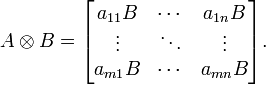
еҰӮжһңAжҳҜдёҖдёӘ m x n зҡ„зҹ©йҳөпјҢиҖҢBжҳҜдёҖдёӘ p x q зҡ„зҹ©йҳөпјҢе…ӢзҪ—еҶ…е…Ӣз§ҜеҲҷжҳҜдёҖдёӘ mp x nq зҡ„зҹ©йҳөпјҢиЎЁзӨәдёәеҰӮеӣҫжүҖзӨәпјҡ
the kronecker product of a row vector and a column vector is essentially their outer productгҖӮ
|
1 2 3 4 5 6 |
>> (kron(U(:,1)',V(:,1))*E(1,1))' ans = 2.0752 1.4487 2.7017 3.9606 2.7649 5.1563 |