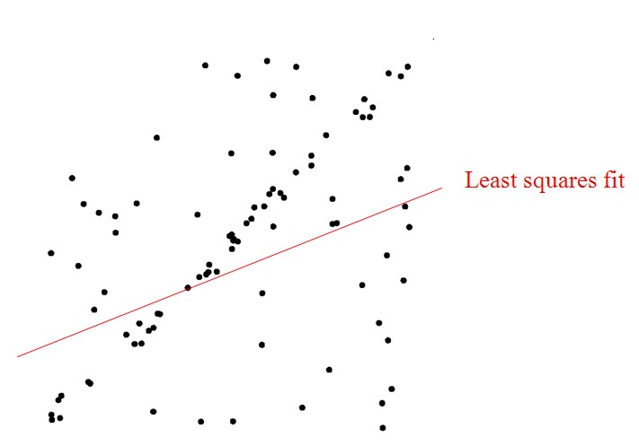
例子:在一组数据点中找到一条最适合的线。 假设,此有一组集合包含了内群(inliers)以及离群(outliers),其中内群为可以被拟合到线段上的点,而离群则是无法被拟合的点。
传统的统计方法都会隐含假设:超过一半的数据点满足参数模型。而实际数据点,很小一部分的outliers就会导致糟糕的性能。如果inliers占大多数,outliers只是很少量时,我们可以通过最小二乘法或类似的方法来确定模型的参数和误差。如果无效数据很多(比如,超过了50%的数据是无效数据)。

给定两个点 与
与 的坐标,确定这两点所构成的直线。对于输入的任意点
 ,判断它是否在该直线上。
 ,
, 。直线表达式为
 。我们想确定参数
 与
与 的具体值,
的具体值, 可以通过与算得。通过实验,可以得到一组
 的测试值。虽然理论上两个未知数的方程只需要两组值即可确认,但由于系统误差的原因,任意取两点算出的a与b的值都不尽相同。我们希望的是,最后计算得出的理论模型与测试值的误差最小。最小二乘法的思想即通过计算最小均方差关于参数a、b的偏导数为零时的值。
在2维情况下,概率分布形式如下:


最小二乘法以估计值与观测值的差的平方和作为损失函数,极大似然法则是以最大化目标值的似然概率函数为目标函数,从概率统计的角度处理线性回归并在似然概率函数为高斯函数的假设下同最小二乘建立了的联系。定义 ,那么
,那么 。
。
假设所有数据满足高斯分布,然而计算机视觉领域的特征/数据一般不遵循这个假设。残差的二次性增长很快,离群点和内群点对于似然概率有相同的贡献。试想一下这种情况,假使需要从一个噪音较大的数据集中提取模型(比方说只有20%的数据时符合模型的)时,最小二乘法就显得力不从心了。
RANSAC是“Random Sample Consensus(随机抽样一致)”的缩写。它可以从一组包含“离群点”的观测数据集中,通过迭代方式估计数学模型的参数。它是一种不确定的算法——在某种意义上说,它会产生一个在一定概率下合理的结果,而更多次的迭代会使这一概率增加。
RANSAC的基本假设是
- “内群”数据可以通过几组模型的参数来叙述其分布,而“离群”数据则是不适合模型化的数据。
- 数据会受噪声影响,噪声指的是离群,例如从极端的噪声或错误解释有关数据的测量或不正确的假设。
- RANSAC假定,给定一组(通常很小)的内群,存在一个程序,这个程序可以估算最佳解释或最适用于这一数据模型的参数。
|
1 2 3 4 5 6 7 8 9 10 |
输入: 一组观测数据(往往含有较大的噪声或无效点),一个用于解释观测数据的参数化模型 n -所需的最小数据点个数来拟合模型 k -算法允许的最大迭代次数 t -用于决定数据是否适应于模型的阀值 d -判定模型是否适用于数据集的数据数目 输出: best_model —— 跟数据最匹配的模型参数(如果没有找到好的模型,返回null) best_consensus_set —— 估计出模型的数据点 best_error —— 跟数据相关的估计出的模型错误 |
RANSAC通过反复选择数据中的一组随机子集(从数据中随机选择m个点)来达成目标。被选取的子集被假设为内群点,并用下述方法进行验证:
- 有一个模型适应于假设的内群点,即所有的未知参数都能从假设的内群点计算得出。
- 用得到的模型去测试所有的其它数据,如果某个点适用于估计的模型(误差小于t),认为它也是内群点。
- 如果有足够多的点被归类为假设的内群点,那么估计的模型就足够合理。
- 然后,用所有假设的内群点去重新估计模型(譬如使用最小二乘法),因为它仅仅被初始的假设内群点估计过。
- 最后,通过估计内群点与模型的错误率来评估模型。
- 上述过程被重复执行固定的次数,每次产生的模型要么因为内群点太少而被舍弃,要么因为比现有的模型更好而被选用。
伪代码
|
1 2 3 4 5 6 7 8 9 10 11 12 13 14 15 16 17 18 19 20 21 22 23 |
iterations = 0 best_model = null best_consensus_set = null best_error = 无穷大 while ( iterations < k ) maybe_inliers = 从数据集中随机选择m个点 maybe_model = 适合于maybe_inliers的模型参数 consensus_set = maybe_inliers for ( 每个数据集中不属于maybe_inliers的点 ) if ( 如果点适合于maybe_model,且错误小于t ) 将点添加到consensus_set if ( consensus_set中的元素数目大于d ) 已经找到了好的模型,现在测试该模型到底有多好 better_model = 适合于consensus_set中所有点的模型参数 this_error = better_model究竟如何适合这些点的度量 if ( this_error < best_error ) 我们发现了比以前好的模型,保存该模型直到更好的模型出现 best_model = better_model best_consensus_set = consensus_set best_error = this_error 增加迭代次数 返回 best_model, best_consensus_set, best_error |

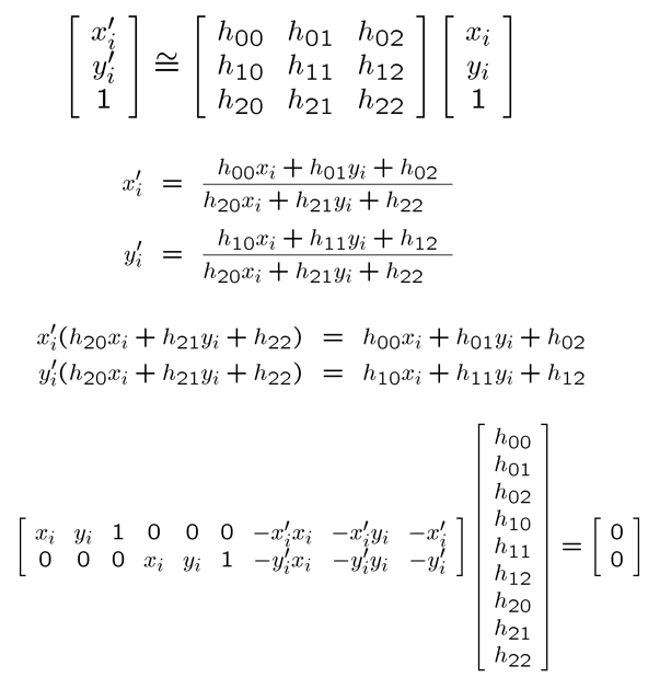
例子:求取Homography单应矩阵
在计算机视觉的背景下,2d affine是2D homography的子集。
从几何意义上讲,2D homography是用来计算一堆在同一个三维平面上的点在不同的二维图像中的投影位置的,是一个一对一的映射。2D affine是2D homography的一个特例,它对应着的情况是这个三维平面在无穷远。从代数特性上讲,2D homography是一个rank=3或者说可逆的矩阵,一般可以表示为:
|
1 2 3 |
H11 H12 H13 H21 H22 H23 H31 H32 1 |
Affine是它的简化形式,不但可逆而且第三行没有未知数:
|
1 2 3 |
A11 A12 A13 A21 A22 A23 0 0 1 |
计算homography(线性解)需要4对不共线的点(8个点),计算affine只需要3对不共线的点。一般要用RANSAC这个方法来得到精确、鲁棒的结果。affine一般比homography更稳定一些,所以可以先计算affine,然后再用affine作为homography的初始值,进行非线性优化(比如Levenberg Marquardt)。homography可以用来计算一幅图像中的不同平面的变换,也可以是不同图像中的同一个平面的变换。affine是它的特殊情况。

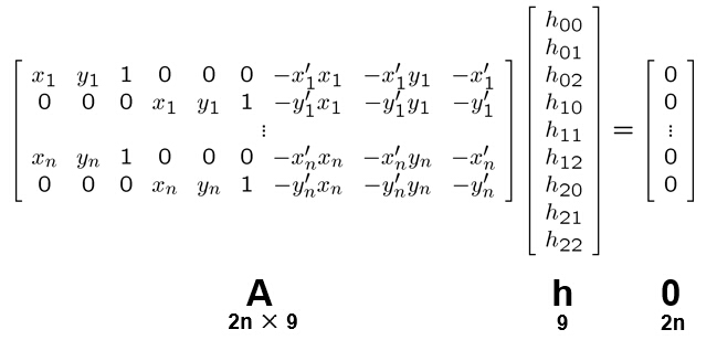
定义最小二乘问题:
- Since h is only defined up to scale, solve for unit vector

- Solution: = eigenvector of
 with smallest eigenvalue
 - Works with 4 or more points(4对点)
|
1 2 3 4 5 6 7 8 9 10 11 12 13 14 15 16 17 18 19 20 21 22 23 24 25 26 27 28 |
function H = solveHomo(pts1,pts2) % H is 3*3, H*[pts1(:,i);1] ~ [pts2(:,i);1], H(3,3) = 1 % the solving method see "projective-Seitz-UWCSE.ppt" n = size(pts1,2); A = zeros(2*n,9); A(1:2:2*n,1:2) = pts1'; A(1:2:2*n,3) = 1; A(2:2:2*n,4:5) = pts1'; A(2:2:2*n,6) = 1; x1 = pts1(1,:)'; y1 = pts1(2,:)'; x2 = pts2(1,:)'; y2 = pts2(2,:)'; A(1:2:2*n,7) = -x2.*x1; A(2:2:2*n,7) = -y2.*x1; A(1:2:2*n,8) = -x2.*y1; A(2:2:2*n,8) = -y2.*y1; A(1:2:2*n,9) = -x2; A(2:2:2*n,9) = -y2; [evec,~] = eig(A'*A); H = reshape(evec(:,1),[3,3])'; H = H/H(end); % make H(3,3) = 1 end |
|
1 2 3 4 5 6 7 8 9 10 11 12 13 14 15 16 17 18 19 20 21 22 23 24 25 26 27 28 29 30 |
function [H corrPtIdx] = findHomography(pts1,pts2) % [H corrPtIdx] = findHomography(pts1,pts2) % Find the homography between two planes using a set of corresponding % points. PTS1 = [x1,x2,...;y1,y2,...]. RANSAC method is used. % corrPtIdx is the indices of inliers. coef.minPtNum = 4; coef.iterNum = 30; coef.thDist = 4; coef.thInlrRatio = .1; [H corrPtIdx] = ransac1(pts1,pts2,coef,@solveHomo,@calcDist); end function d = calcDist(H,pts1,pts2) % Project PTS1 to PTS3 using H, then calcultate the distances between % PTS2 and PTS3 n = size(pts1,2); pts3 = H*[pts1;ones(1,n)]; pts3 = pts3(1:2,:)./repmat(pts3(3,:),2,1); d = sum((pts2-pts3).^2,1); end |
|
1 2 3 4 5 6 7 8 9 10 11 12 13 14 15 16 17 18 19 20 21 22 23 24 25 26 27 28 29 30 31 32 33 34 35 36 37 38 39 40 41 42 43 44 45 46 47 48 49 50 51 52 53 54 55 56 57 58 59 60 61 62 63 64 65 66 67 68 69 70 71 72 73 74 75 76 |
function [f inlierIdx] = ransac1( x,y,ransacCoef,funcFindF,funcDist ) %[f inlierIdx] = ransac1( x,y,ransacCoef,funcFindF,funcDist ) % Use RANdom SAmple Consensus to find a fit from X to Y. % X is M*n matrix including n points with dim M, Y is N*n; % The fit, f, and the indices of inliers, are returned. % % RANSACCOEF is a struct with following fields: % minPtNum,iterNum,thDist,thInlrRatio % MINPTNUM is the minimum number of points with whom can we % find a fit. For line fitting, it's 2(2对). For homography, it's 4(4对). % ITERNUM is the number of iteration, THDIST is the inlier % distance threshold and ROUND(THINLRRATIO*n) is the inlier number threshold. % % FUNCFINDF is a func handle, f1 = funcFindF(x1,y1) % x1 is M*n1 and y1 is N*n1, n1 >= ransacCoef.minPtNum % f1 can be of any type. % FUNCDIST is a func handle, d = funcDist(f,x1,y1) % It uses f returned by FUNCFINDF, and return the distance % between f and the points, d is 1*n1. % For line fitting, it should calculate the dist between the line and the % points [x1;y1]; for homography, it should project x1 to y2 then % calculate the dist between y1 and y2. minPtNum = ransacCoef.minPtNum; iterNum = ransacCoef.iterNum; thInlrRatio = ransacCoef.thInlrRatio; thDist = ransacCoef.thDist; ptNum = size(x,2); thInlr = round(thInlrRatio*ptNum); inlrNum = zeros(1,iterNum); fLib = cell(1,iterNum); for p = 1:iterNum % 1. fit using random points sampleIdx = randIndex(ptNum,minPtNum); f1 = funcFindF(x(:,sampleIdx),y(:,sampleIdx));%3*3的矩阵,由最小二乘求解得到 % 2. count the inliers, if more than thInlr, refit; else iterate dist = funcDist(f1,x,y);%x*H=y,计算一个点由H矩阵映射后得到的估计点与真实点的误差 inlier1 = find(dist < thDist);%由阈值找出内群点 inlrNum(p) = length(inlier1);%存放每一轮迭代取得的内群点个数 if length(inlier1) < thInlr, continue; end fLib{p} = funcFindF(x(:,inlier1),y(:,inlier1));%存放每一轮迭代找出的H矩阵 end % 3. choose the coef with the most inliers [~,idx] = max(inlrNum);%找出最大的内群点个数对应的迭代轮数 f = fLib{idx};%相应的H矩阵 dist = funcDist(f,x,y); inlierIdx = find(dist < thDist);%再计算一遍内群点数目,这里为10个 end |
|
1 2 3 4 5 6 7 8 9 10 11 12 13 14 15 16 17 18 19 20 21 |
function index = randIndex(maxIndex,len) %INDEX = RANDINDEX(MAXINDEX,LEN) % randomly, non-repeatedly select LEN integers from 1:MAXINDEX if len > maxIndex index = []; return end index = zeros(1,len); available = 1:maxIndex; rs = ceil(rand(1,len).*(maxIndex:-1:maxIndex-len+1)); for p = 1:len while rs(p) == 0 rs(p) = ceil(rand(1)*(maxIndex-p+1)); end index(p) = available(rs(p)); available(rs(p)) = []; end |
参考资料:
1)http://dichild.com/?cat=1
2)https://en.wikipedia.org/wiki/RANSAC
3)百度文库“计算机视觉中的几何学”
4)http://blog.sina.com.cn/s/blog_49babfed0100pq7y.html
5)http://www.opencv.org.cn/opencvdoc/2.3.2/html/doc/tutorials/features2d/feature_homography/feature_homography.html opencv 源码 待研究